This is a quick update on our flagship product development, PMU-001. Since October 2024, we put great effort in developing it. The PMU-001 USB device is intended for electricians that need a portable and reasonably affordable field device which provides the following features :
Robust GPS based synchrophasor measurement, IEEE Std C37.118-2005 compliant with network bindings.
6 channel analysis (3 voltage channels, 3 current channels, 2 auxiliary channels)
4 quadrant power analysis
Positive, negative and zero sequence vector decomposition
logging and real-time (within standard delay requirement) equispaced sampling of frequency deviation from nominal mains
Harmonics analysis and THD display and logging
waveform logging
USB 2.0 high speed device, hardware sampling rate 48 ksps.
Lightweight NCURSES interface allowing use across low speed / character based tty
Integrated class 0.1 voltage measurement transformers with secondary DAC TVS protection / clamping on top of internal DAC protection.
1000V AC transformer winding voltage tolerance.
Line to Line or Line to Neutral voltage measurements (120V up to 240V AC / 208V AC to 400V AC nominal voltage +15% tolerance)
It leverages the power of a personal computer for high level analysis, reducing hardware costs, the software payload is C++ based and works on Linux distributions. Microsoft Windows porting is planned in the future.
A fully functional hardware and software prototype is planned for Q3 2026.
Most of the work is now dedicated on GPS disciplining and TCXO clocking, as well as cross channel analysis for four quadrant measurement, and delay vs filtering efficiency real time tuning. IEEE Std C37.118-2005 compliance will require rigorous conformity testing and calibration. At that time, a crowdfunding effort with pre-order priority will be put into effect, allowing trade electricians to have priority access to the device in the beta phase.
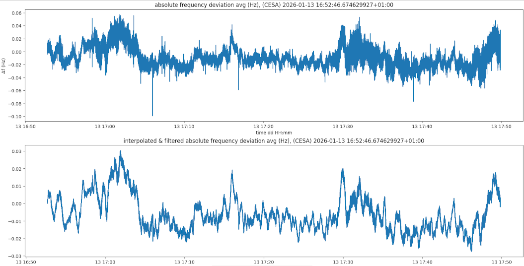
Here are some video and screen capture teasers :
NCURSES display of frequency deviation, ROCOF, harmonic analysis, amplitude analysis, and synchrophasor data. Single phase to neutral display.top chart : raw frequency deviation measurements at 100 Hz sampling rate; bottom chart LP filtered at 10 Hz cutoff frequency and PCHIP interpolated/equispaced frequency deviation measurements. Network PMU connection to PMU-001 using GPA PMU Connection Tester tool, displaying a single voltage channel synchrophasor and frequency measurements.
We wish everyone a fruitful 2026 year. Stay tuned for updates !
This article documents the development and testing of the Linux driver module and the interface between the Raspberry Pi GPIOs and the AD7606-F4 development board. The AD7606-F4 is based on the AD7606-8, The 8 channel version of the AD7606, true bipolar, ±5V / ±10V input range, 16 bit, with 1 to 64 hardware oversampling, simultaneous sampling ADC. The driver development effort is focused on the 16 bit parallel interface mode instead of SPI. It leverages the Linux industrial IO layer. The goal is mainly to characterize maximum achievable sample rate / triggering rate, as well as sample loss and jitter induced by kernel burden and scheduling, depending on triggering rate, while using “worst case” interfacing. No backend IC is used to perform hardware protocol management and hardware buffering in our tests.
Using a small SOC with limited RAM and CPU capabilities also conforms with worst case performance testing, and will allow us to identify the limiting factor of such a setup.
Initial driver development was performed by Analog Devices and the driver maintainer and is available in the linux kernel source. It lacked however several features, but offered a good starting base for a fully functional driver. The available driver is split into two source files, one for the parallel interface and one for the SPI interface.
We will explore the various methods of interacting with GPIOs inside the kernel module, as to improve the conversion/read cycle time for all channels.
The maximum sampling speed is mainly dictated by the kernel load, as a direct interfacing of the AD7606 to the Raspberry Pi requires handling interrupts at the sampling speed. The main limiting factor however seems to be the gpiod_set_raw_value() execution time, and thread synchronization between the trigger handler and the IRQ handling callback, limiting sampling rate short of 8 ksps.
IIO provides a mechanism, called backend, to interface signaling (such as conversion start, handling of IRQ and first channel read detection) by an intermediary device such as an IP core. This provides also hardware buffering so that IIO gets data from the hardware buffer in chunks, so that IRQ loading to the kernel is lowered.
Note that besides kernel performance limitations, high sampling rates also require application of common hardware interfacing best practices, such as :
Minimising trace or cable length to minimize loop inductance
Keeping same trace length, but it is secondary since the baud rate is still conservative even at the max rate allowed by the ad7606, dicated by the minimum timings specified in the datasheet.
Adding small values resistors such as 51 ohm on the lines to minimize ringing
Adding guard traces grounded on one side to reduce crosstalk and inductive coupling between data lines, and between signalling lines.
The GPIO pin layout vs the line pin layout on the AD7606-F4 dev board we are using cannot allow the use of a 40 pin ribbon cable such as those use for ATA UDMA transfer, as it would require crossing over lines, so a mating PCB or hat design is required.
Low sampling rates can be achieved using standard dupont cables, and assessing the sampling rate limits for such a solution is one of the goals of this article.
Note that using 20cm dupont pin cables, without current/ringing limiting resistors as inductive dampers, it is highly improbable to reach sampling rates such as 48 ksps as found on audio interfaces using backend-less interfacing. Pushing the sampling rate above 8 ksps would mainly require, in that order :
MMIO for signalling (CONVST, CS/RD strobes) instead of reliance on gpiod_set_raw_value()
Using try_wait_for_completion() in a preempt_disable() / preempt_enable() context
A more robust and faster SOC, with dual core at least to enable IRQ pinning on a core
Using a RT linux kernel
A hat or PCB mating interface to improve signal integrity
However, determining the practical limit of such a solution is useful as it is the most cost effective and fast way to interface a Raspberry Pi or other SOC to perform ADC operations using the industrial IO layer.
The Github link to the kernel module driver and its associated helpers is available at the very end of this article.
General interfacing using the parallel interface layer.
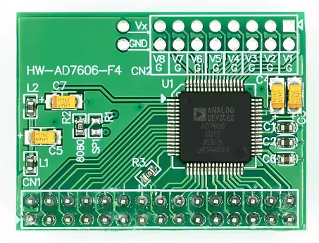
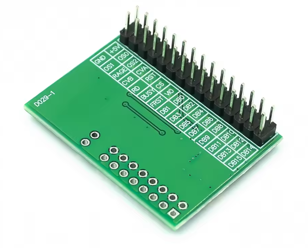
The AD-7606-F4 development board we used and available on Aliexpress or other chinese marketplaces has a small footprint. The development board we got does not exposes the standby pin, and was factory set for parallel interface transfer through a SMD resistor on the 8080 pad identified by silkscreen marking. Swapping the resistor into the SPI pad would obviously enable SPI mode. Note that the AD7606, to achieve full sampling rate performance for SPI requires dual SPI mode.
In parallel mode, the signalling requires at least the following lines connected between the AD7606 and the Raspberry Pi :
We will use the Raspberry Pi (host interface, as the reference for IN/OUT specification)
CONVSTA/CONVSTB : these two lines can be tied together into a single GPIO on the Raspberry Pi. These are OUT pins. They are strobed low to signal that we want to initiate a conversion. if the pins are strobed low at the same time, all 8 channels are simultaneously sampled, if strobed independently, they allow sampling of the first 4 and last 4 channels independently, the sampling delay allows compensation of group delays induced by filters or CT vs VT in power grid measurements.
BUSY : IN pin, the falling edge indicates end of conversion and signals the SOC (through GPIO IRQ management) that it is ready for data reading of all channels.
FRSTDATA : IN pin, this signals the readout of the first channel, so that there are no channel alignment issues : if FRSTDATA level is not high when the SOC reads the first channel as the driver internal state indicates, or if FRSTDATA level is high when the SOC expects to read subsequent channels, it should be treated as an IO error and all channels samples should be discarded from the read cycle. The AD7606 should be reset through the RESET pin. Monitoring RESET events from this condition is recommended in the debugging phase, as it indicates potential hardware interfacing problems and instability. If too much FRSTDATA mismatches occur, try increasing timing delays for all pin strobes.
RESET : OUT pin, commands the AD7606 to reset. Used if an inconsistent state is detected, see above. A reset event will lower sampling rate, as the interface needs some time after the reset to be fully operational. Reset is also called in the probe function at device initialization as the ad7606 should be reset after power-up or resume from standby.
CS/RD : OUT pins. tells the AD7606 to shift next channel into the parallel interface registers, and select the AD7606 if they are stacked on the same parallel line. if exactly one AD7606 is present on all lines, then CS/RD can be strobed simultaneously (linked mode). Signaling is easier this way, as independent CS/RD management gives a slightly different timing protocol. Refer to the datasheet for independent management of CS/RD. Our driver uses linked CS/RD mode, but our tests were performed with two separate lines driven concomitantly. (GPIO levels set on two pins synchronously)
The remaining pins, RANGE, 0S0, 0S1, 0S2 are configuration pins used to select the input voltage range specification (+-5V or +-10V) and OSx pins are used to set the bits that select the oversampling mode.
The AD7606-F4 dev board does not expose the STBY pin on the 40 pin header.
The “VO” pin on the AD7606-F4 corresponds to the AD7606 Datasheet pin mnemonic “VDRIVE“. This pin should be connected to the 3.3V line of the Raspberry Pi. This line supplies the logic power and sets the levels used on the data pins, FRSTDATA, and BUSY.
In our setup, leftover pins are GPIO0, GPIO1 and GPIO27. GPIO0 and GPIO1 are reserved and used by external EEPROM hats, they can be reclaimed using the force_eeprom_read=0. This prevents EEPROM boot time operations on these pins. We did not test these pins in our use case. GPIO27 is leftover.
If CS/RD were tied, another pin would be returned to the pool of free pins, making 4 leftover pins.
Oversampling can be configured statically to reclaim 3 more pins
In order to avoid interface conflicts, raspi-config or edition of /boot/firmware/config.txt should be performed to disable pin functions such as UART, SPI, I2C, 2wire, EEPROM.
Parallel interface Data Pins
The AD7606 provides byte mode parallel transfers besides word parallel mode, in byte mode, each channel data is supplied to the host through two successive data reads. (MSB/LSB or LSB/MSB). This mode halves the maximum achievable data rate, but allow recovery of 8 pins for other uses.
The 16 bit (word) data transfer rate, require a single CS/RD or RD strobe per channel read, at the expense of using a full 16 pin block. This is the mode we used in our demo.
Note that data line pin mapping between the host and AD7606 should be contiguous and ordered to prevent unnecessary bit reordering and masking. GPIO order is determined by the BCM GPIO pin nomenclature, not pin ID number.
Bit shifting is required however if the data lines start at an offset, that is, if they don’t start at GPIO0.
In our use case, we used the GPIO8 to GPIO23 range as the 16 parallel GPIO lines. ARM architecture is optimized to read 32 bits, with correct alignment when using MMIO (memory mapped IO), which means, in our case, reading 4 bytes at GPIOLEV0 offset, and extracting the 2 center bytes, which requires a simple bit shift, bit mask and cast to u16 operation. for MMIO, we used the industry tested readl() MMIO function, although recent kernel practices seem to shift towards the use of ioread32(), Which seems to work well too in our tests.
MMIO in kernel space on the Raspberry Pi Zero W.
Using gpiod_get_* functions for parallel data transfers is grossly inefficient. That is why a more direct path is required for transfers, which is achievable using memory mapped IO. This will be tested in future revisions of this article.
Basically, performing MMIO requires knowing the Physical memory mapping base address of the BCM8235 bus address. On Raspberry pi Zero W, it is 0x20200000. (not 0x7…, as indicated as base on the BCM8235/6 datasheet : this is the BUS address, and not 0x32…. : this is the physical memory mapping on newer Raspberry pi Boards such as Pi2/3/4)
Note that the pinctrl tool can be used to ascertain the physical memory mapping base address. Here is the trap however : 0x32000000 base address seems to work in our case to get GPIO levels using a mmap wrapper with Python, since it reflected pin changes, but it did not work in kernel space, so this address base is misleading.
However, The correct 0x202000000 physical memory address base cannot be accessed directly in kernel or user space though. It needs another remapping operation into kernel virtual memory address space.
This is where the request_memory_region() and ioremap() functions come into play and shall be used in the kernel driver module.
request_memory_region() reserves the physical memory region for ioremap(), and prevents any outside access from kernel or user space, which could lead to instabilities and conflicts. Once the requested memory region is allocated to the kernel module drive through the former call, any other request, read or remap operation will result in an error, such as EBUSY.
This is also why disabling conflicting functions such as I2C, SPI, UART, 2wire, EEPROM and consorts that would conflict with the module is required
In our case, we disabled all of the above mentioned functions.
Device Tree Overlays
The driver needs to know which pins to use and which MMIO address space to use. The current best practice is to use only device tree overlays that provide platform specific and implementation specific GPIO pin mapping and MMIO base address information. Using .c or header files as driver board configuration files is a deprecated and discouraged practice, especially in loadable/unloadable (not kernel integrated) modules.
This is why writing a device tree (dts file) overlay is mandatory.
The device tree provides signalling and configuration pin information, as well as data lines pins declaration. The signalling and configuration pin information is used by GPIOd_* functions.
Although data line pins are used by MMIO, which does not use GPIOd_* functions for data transfer, the pin declarations as an array of pins in the device tree overlay is required for configuration of these data line pins as INPUTS, which is done once in the module .probe() callback function, and this step uses GPIOd_set functions for mode configuration.
Configuration of the physical base address used to access GPIOLEV0 registers and data transfer, so that request_mem_region() and ioremap() get the required base address information and number of memory pages to remap is done through the “reg” device tree property.
reg = <0x20200000 0x00004096>;
the first hexadecimal number is the physical memory base address of the GPIO peripheral, and the second number is the number of bytes to be used in request_mem_region() and ioremap() functions.
Note that ARM paging requires at least 4 bytes as size, in our case we mapped a full SZ_4K region, at it is usually done in other similar drivers. The start address needs to be aligned at 4 bytes, which is the case as it is divisible by 4. The total GPIO address space is x bytes.
the “adi,” prefix encountered in properties can be seen as a namespace information (Analog Devices manufacturer), and is used to avoid ambiguous / property name conflicts with other existing device tree properties at the time of dtoverlay loading. This is preferable since some common tokens such as ‘reset’ may already be used.
Pull up / Pull down configuration
Standard pin definitions <&gpio pin_number flags> as pin desc definitions used by the ad7606 are not sufficient to specify the configuration of the internal pulls. These need to be specified as the brcm2835 device level, and referenced by the ad7606 device tree fragment. Pull ups / Pull down not only allow the logic state to settle if the driving side is in high-z mode such as the tri-state FRSTDATA pin, preventing undefined behaviour, they also allow quicker rise and fall edge timings, which is a requirement for high speed transfers.
The device tree, with a preprocessing step. the dts files get pre-processed into a dts.preprocessed file, which itself gets compiled into a binary device tree object (dtbo) that can be used by device tree overlay loading functions such as dtoverlay or dtoverlay statements in the Raspberry Pi /boot/firmware/config.txt
The driver itself, made from one c file and one header files (ad7606_par.c and ad7606.h)
obj-m+=ad7606_par.oCFLAGS_ad7606_par.o:= -UDEBUGEXTRA_CFLAGS+= -fno-inlineall: module dt echo Built Device Tree Overlay and kernel modulemodule: make -C /lib/modules/$(shell uname -r)/build M=$(PWD) V=1 modulesdt: ad7606.dts cpp -nostdinc -I /usr/src/linux-headers-$(shell uname -r | sed 's/-rpi-v[0-9]*//')-common-rpi/include/ -I arm64 -undef -x assembler-with-cpp ad7606.dts ad7606.dts.preprocessed dtc -@ -Hepapr -I dts -O dtb -o ad7606.dtbo ad7606.dts.preprocessedclean: make -C /lib/modules/$(shell uname -r)/build M=$(PWD) V=1 clean rm -rf ad7606.dtbo ad7606.dts.preprocessed
Module Loading helper bash script
The file load.sh is used as helper to load the device tree and kernel driver, as well as its dependencies. In a final driver and its installation procedure, the dependencies are usually stored as lines in a dependency file, .dep.
At the time of writing this article, distribution effort was not yet done, and so it is outside the scope of the article. Which means that modprobe calls in the correct order have to be done to load the required dependencies.
Those are :
industrialio
iio-trig-hrtimer
industrialio_triggered_buffer
Then, the hrtimer0 instance is created as it will be subject to validation by our driver module validate trigger function.
following is the DT overlay load and the kernel module load. The remaining calls are used to configure the sample buffer, triggered buffer sampling frequency (managed by iio hrtimer), and buffer enable at the end, with a real time read of the iio device by using dd.
Commented calls are used for ftrace profiling, to minimize dev_dbg overhead.
#!/bin/bashsudomodprobeindustrialio# load industrial io kernel modulesudomodprobeiio-trig-hrtimer# load hrtimer industrial io kernel modulesudomodprobeindustrialio_triggered_buffer# load industrial triggered buffer kernel modulesudomkdir/sys/kernel/config/iio/triggers/hrtimer/hrtimer0# configure one hrtimer instancesudodtoverlay-vad7606.dtbo#load compiled device tree snippet with ad7606 pin to rpi configsudoinsmodad7606_par.ko#load ad7606 driver modulesudosh-c"echo 10.0 > /sys/bus/iio/devices/trigger0/sampling_frequency"#sets triggered sampling frequency to 10 spssudosh-c"cat /sys/bus/iio/devices/trigger0/name > /sys/bus/iio/devices/iio\:device0/trigger/current_trigger"# configure the ad7606 iio device to use the hrtimer0 instancesudosh-c"echo 1 > /sys/bus/iio/devices/iio\:device0/scan_elements/in_voltage1_en"# configure the triggered buffer to output a single channel, the second channel. (channels are 0 indexed)cat/sys/bus/iio/devices/iio\:device0/in_voltage1_raw#output raw value for testing. The first sample is usually invalid, this needs debugging.cat/sys/bus/iio/devices/iio\:device0/in_voltage1_raw#gets another sample, this value should be ok.#sudo vclog -m#Make sure tracing is disabled during tracing reconfiguration#echo "disabling tracing and current_tracer"#sudo sh -c "echo 0 > /sys/kernel/debug/tracing/tracing_on"#sudo sh -c "echo nop > /sys/kernel/debug/tracing/current_tracer"#sudo sh -c "echo ad7606_* > /sys/kernel/debug/tracing/set_ftrace_filter"#echo "ad7606_* written to set_ftrace_filter"#sudo sh -c "echo function_graph > /sys/kernel/debug/tracing/current_tracer"#sudo sh -c "echo 2 > /sys/kernel/debug/tracing/max_graph_depth"#echo "set max_graph_depth to 2"#sudo sh -c "echo 1 > /sys/kernel/debug/tracing/tracing_on"#echo "function_graph enabled in current_tracer, and enabling tracing "echo"now enabling device buffer"sudosh-c'echo 1 > /sys/bus/iio/devices/iio\:device0/buffer0/enable'echo"buffer enabled"#echo "reading trace_pipe in 2 secs"#sleep 2#sudo sh -c "cat /sys/kernel/debug/tracing/trace_pipe > /root/trace.log"echo"will now output raw, aligned sample bytes from buffer device"sudosh-c"dd if=/dev/iio\:device0 bs=20 iflag=fullblock | hexdump"
Performance testing
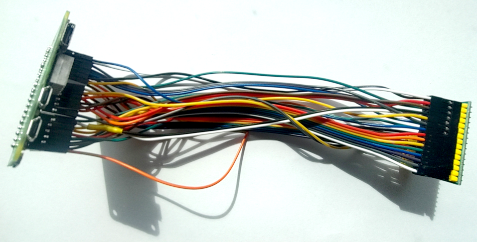
The following picture shows the testing conditions. Such a crude interface is useful for getting “worst case performance” data, which are useful in setups where the AD7606 must be up and running in the least amount of time and least amount of money (from placing order to sampling, using off the shelf components)
When using MMIO for data transfer, and gpiod_* functions for signalling CONVSTx, CS/RD, and reading FRSTDATA, the gpio_d* function calls will be bottleneck. A full convst/read cycle takes around 60us. In that case, the maximum theoretical sampling rate would be 15 ksps. We expect that 8 ksps could be a conservative max practical limit accounting for kernel IRQ burden. Using full MMIO would probably help push the limit higher, if care is given to disable as much system noise as possible (such as HDMI, videocore drivers, bluetooth, framebuffers, etc). A more capable raspberry pi such as 3/4 which have more than 1 core, could use IRQ pinning to help such a fully MMIO optimized driver to work at maximum speed, provided a mating board or a full fledged ad7606 hat is used for hardware performance.
The FRSTDATA channel synchronization mechanism and error rate
The tristate (High-Z, HIGH/LOW) FRSTDATA input is used to signal that the first channel is ready to be read. This hardens the transfer protocol as the sample frames remains aligned, that is, the channels do not get misaligned in the output buffer. Algorithmically, a boolean “first-channel” is set to true at the beginning of the samples read process. it is compared to the level of the FRSTDATA pin, and the comparison should branch to true. The boolean is then set to false and compared to FRSTDATA level for the remaining channels and should also branch to true. If there is a mismatch, sample readout is aborted, and a RESET is sent to the ad7606, through the ad7606_reset functions, and the that were abl where the internal driver pin state is also reset so that the whole conversion/readout cycle can be resumed.
The FRSTDATA pin is a good indicator of hardware stability and hardware interfacing quality. Lowering strobe cycle periods and overall timing delays will typically increase the number of spurious FRSTDATA states and subsequent resets, especially when reaching the limits of hardware interface stability, which can happen well before the timing limits of ad7606 datasheet when using an ad-hoc long Dupont header pins cable interface. In our case, the IRQ load on the kernel as well as the gpiod_set_* command timing overhead are the bottleneck.
For reference, This is the average spurious FRSTDATA error rate over 1 hour sampling at various sampling rates. Test conditions : Raspberry Pi Zero W, 20 cm Dupont header cables, internal pulls used on all input pins, no current limiting resistors.
1000 sps = 2.44 %
2000 sps = 2.74 %
4000 sps = 3.08 %
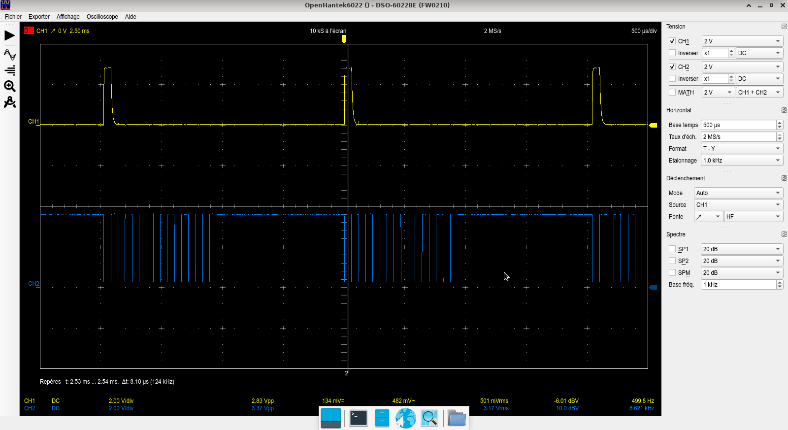
The following oscilloscope capture shows the FRSTDATA channel read synchronization signal on CH1 and the linked mode CS/RD pulse strobes used to latch all channels (8) data into the parallel interface lines
FRSTDATA (CH1) and CS/RD (CH2)
timer trigger callback function performance
We tested three code combinations to jauge performance
gpiod_set_raw_value() functions for CONVST and CS/RD strobes + wait_for_completion_timeout() synchronization.
MMIO based CONVST and CS/RD strobes + try_wait_for_completion() after usleep_range(5,10)
MMIO based CONVST and CS/RD strobes + wait_for_completion_timeout()
at a sampling rate of 100sps, with an incompressible strobe time of 200ns.
The run time of the callback , averaged over 500 trigger calls are
(1) = 122 µs
(2) = 108 µs
(3) = 100 µs
In our case the best execution time of the trigger handler was on average 100us, using 100ns timing for pin strobe delays. Note however, that most of the time spent is not accounted from these timing delays, but by the slowness of the gpiod_set_* functions, MMIO write to a lesser degree, buffer publishing to the IIO stack and IRQ thread synchronization to trigger handler using completions. The CONVSTA/B to BUSY falling edge published in the datasheet is specified as 5us, which is a minor contribution to the overall cycle. Note that wait_for_completion_timeout() puts the thread on the wait queue, and the IRQ handles completion using complete(), which resumes the trigger handler thread, this has probably quite some overhead, but is safe in IRQ contexts, It seems however that for a 5 µs conversion time, there is no performance gain, but loss, using the usleep_range(5,10) + try_wait_for_completion() combination. Using MMIO gives a moderate performance boost. Overall the limiting factor seems to be MMIO performance and iio_push_to_buffers_with_timestamp() performance, which could improve with faster cores and memory. Compared to older buses such as PIO ATA (Programmed IO mode, that does not leverage DMA) the maximum throughput would be 8 * 2 bytes / 100 µs = 160 kB/s, which is still 20 times slower than PIO Mode 0. Thus continuing effort on investigating MMIO performance and IIO call responsivity is required, as several studies have shown, with oscilloscope proof, that Mhz frequency range strobes are possible on Rpi, albeit using tight loops MMIO strobes. A further investigation on each code component contribution inside the callback would allow a precise evaluation of performance, and using an oscilloscope instead of relying on kernel timestamp tracing, which have a non negligible overhead.
wait_for_completion_timeout() also returns a non zero integer if timeout is not reached, representing the remaining jiffies in the supplied timeout. It can thus be used to check the time waited by a simple subtraction. Note that with a kernel “HZ” value of 100, one jiffy is 10 msec, which resolution is too low to provide any sensible performance metric for tuning. Any value returned different of the supplied timeout would only inform of a severe contention of IRQ mishandling.
At 100 us conversion/read cycle, the theoretical maximum sampling rate is short of 10 ksps.
Maximum toggling speed using MMIO in tight loop
As noted in (1), the maximum toggling speed on Raspberry Pi 1 (using a preformatted 32 bits mask) “Direct output loop to GPIO” was stated to be 22.7 Mhz, backed by oscilloscope readings.
It looks like the code was ran from user space using /dev/mem mapping.
We managed to get a speed of 24.9 Mhz from kernel space, using the boot config CPU boost (overclock) and a proper heatsink. Although it is not backed from oscilloscope reading to reflect waveform quality yet, though the following code, using the GPIO “standby” pin in our module, as it is not used by the AD7606-F4 development board.
While this approach can get you sampling 8 channels fast, it mainly limits to slow sampling requirements and cannot guarantee equispaced sampling. On the other hand, no hardware buffering means the latency is minimal, and it also builds on top of IIO seamlessly.
For serious speeds a fully integrated acquisition system featuring a MCU and the AD7606, and a convenient interface such as USB is preferable.
An AD7606 development board is 7 to 11 USD pu (Aug 2025).
A full-fledged USB acquisition system based on AD7606 is expected to cost 50 to 60 USD p.u. (Aug 2025).
Such a system will probably be the focus of our interest in our next article about the AD7606. Stay tuned.
Article updated the 20th of August 2025, reflecting the recent analysis of GPIO performance of Raspberry Pi in user space contexts and Python, vs kernel based contexts using GPIOd_* functions or MMIO, and the suitability of Linux Industrial IO subsystem for such endeavours. DUT pictures were added.
When interfacing a Geiger-Muller device with a MCU or a Raspberry pi, there are mainly two options available :
Use of a high level device, which transfers counter information digitally such as cps, cpm, tube type, stored memory or whatever information the device holds. Some devices may also be able to inform the host of a pulse detection using a low level signaling mode, and perform as a low level device. High level devices may be more or less sophisticated and allow for calibration, unit conversions, dosimetry, or changing settings depending on the tube model and their efficiency characteristics. High count compensation due to dead time may or may not be done, but any serious device should perform such processing. The compensation formulas are dependent on the designer knowledge of the matter and their proprietary choices.
Use of a low level device. Such a device is an analog front end that supplies high voltage to the GM tube, and outputs detected events as pulses on a GPIO pin. The short pulse is usually stretched to a fixed time pulse, with sharp rising and falling edges. It should essentially output a square wave signal, that is easily processed by subsequent A/D stages that are not part of the device itself. Signal output is commonly done via GPIO header pins and/or 3.5 audio jacks. Most also feature a buzzer for direct audio pulse output.
This article is focused on the low level devices and their interfacing with a digital counting platform such as the Raspberry Pi, as it offers maximum processing flexibilityand straightforward interfacing. butfor low count rates only.
Note that for high CPM processing, digital latency effects starts to be significative when using a non real-time OS platform due to operating system overhead (kernel scheduling & pre-emption). Part of this article will deal with mitigation of these unwanted effects.
GM Tube basics.
There are plenty of resources explaining the physics of the GM Tube. We won’t cover them in detail except for the important issue of dead time and how this skew the measured count rate at high levels of ionizing radiation (high count rates). This issue is critical as the device underestimates the count at these regimes. That is, the device is not linear.
The GM Tube is supplied a high enough voltage to work in the Geiger plateau, such as an ionization event triggers a Townsend avalanche and a significant charge is displaced between anode and cathode, and this is seen by the amplifier (either a transistor or an op-amp) as a voltage pulse. This charge displacement is equivalent to a lowering of the impedance of the GM Tube, which induces a voltage drop from the nominal high voltage, as the high voltage source is far from ideal, it can’t source much current and has added resistors. The GM tube and resistors on the high voltage path perform as a voltage divider (with a parallel path to ground, the GM tube – with its impedance lowering during the Townsend avalanche process)
This voltage drop is conditioned to a low voltage (with reference to ground), buffered, and the pulse is stretched to several hundreds of microseconds to a couple of milliseconds, depending on the design and/or tuning. Pulse stretching usually involves stages such as Schmitt triggers and 555 timers
Dead time from the analog front end.
Usually the analog front end circuitry processing exhibits a non-paralyzable dead-time characteristic.
dead time : it means that after a pulse is detected by this front end, any subsequent pulse is not detected during the interval spanning from the registered pulse to the expiration of the dead-time (the pulse stretched “HIGH’ state time, set usually by an analog timer such as a 555.)
non-paralyzable : it means that any townsend avalanche event occuring during that dead-time interval. does not re-trigger the dead time, or at least, it should not. If it does, it would be a poor design choice as dead-time from any processing stage should be minimized as much as possible, and a paralyzable dead-time may extend this duration.
GM Tube intrinsic dead time.
As for the GM tube Townsend avalanche process, it has an intrinsic dead time characteristic that is short but still significative. After a sucessful ionizing event detection, one that triggers a full Townsend avalanche, the tube is unable to detect any other event during the dead time. This dead time is usually in the order of 80 to 200 µs, and is mostly paralyzable : Any event ocurring during that dead time, resets that intrinsic dead time to some extent. For sake of simplicity, we will treat it as a fully paralyzable dead time. In reality, most of the literature agrees that this intrinsic dead time falls in between a paralyzable and non paralyzable model.
We make the supposition that the dead time is a function of the time separation of two subsequent (or more) ionization events, with the limit reaching the nominal dead time as event separation in the time domain goes toward infinity. The precise model of a Townsend avalanche and its practical implementation in a commercial GM tube is outside of the scope of this article.
Thus it follows that the dead-time nominal values from the GM Tube and those of the analog pulse stretch front end are important parameters for count rate compensation.
Analog front end deadtime measurement is quite straightforward in a low count (low background radiation) environment, and can be done by plugging the GM meter jack output to a sound card set at the highest sampling capability, ideally 96ks/s or more. Or better, by using an oscilloscope.
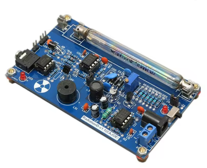
GM Module used for our tests
The following device is widely available on Chinese marketplaces, fully mounted, for around 15 to 20 EUR. It bears the PCB designer silkscreen marking “RadiationD V.1.1(CAJOE)”. It uses two DIP8 555 timers, and one LM358 op-amp.The provided GM tube is a Chinese J305Pr. The three IC are mounted on sockets, allowing for easy replacement. A simple mod could allow tuning the pulse stretching time of the analog front end for better performance in high pulse count environments and for MCU/SOC event processing, at the expense of the audio cue jack output.
Analog front end and audio cue CPM/CPS monitoring considerations
With that DUT in mind, the front end deadtime (the stretched pulse width) was measured at around 2.2ms on average. The reason for such a long deadtime is that it is intended to be processed by the human ear system, a too short pulse would lead to deficient audio cue for low pulse counts such as background radiation monitoring. For high pulse counts, the saturation to constant “high” level from such long pulses piling up would render audio cue high pulse count monitoring ineffective and dangerous, as saturation would provide a constant high level logic output. That is DC and it is converted to a silent state by any speaker or headphone.
That is why a good analog front end used to generate an audio cue signal would use a charge pump pulse to variable voltage conversion stage, such as an LM3907/LM2917 and a VCO to generate an audio tone whose frequency is dependent on the integrated pulse count over n last seconds. A common value for n would be 1 or 60 or more (infinity integration and resettable) for “dosimetric” readings. The integration range could be switch selectable. The transfer function of the VCO (V to f) should be carefully designed so as to provide good audio cues for low up to high count rates, taking into account frequency cut-off of the human ear for older subjects.
The two extreme points on the CPM transfer function (60s integration) could be in the ballpark of :
20 CPM -> 50 Hz
50000 CPM -> 4kHz.
With amplitude compensation accounting for the human ear psychoacoustics, which decrease the sensitivity to high frequency tones and taking into account the risk of ear damage.
A superimposed alarm tone should be used above 50000 CPM to warn the user of unreliable count estimation.
DUT J305Pr intrinsic dead time
As for the intrinsic dead time of a given GM Tube, some are reported in datasheets as an estimation. We could not find one for the J305Pr. Determination of that dead time is not an easy task, in part because the ionization events exhibit a probabilistic distribution (modeled as a Poisson process) – That is, it is hard to control the precise moment when a ionization event will trigger a Townsend avalanche, and relative time to the next incoming gamma-ray or alpha/beta particle that would trigger an avalanche. Best to err to the side of caution and assume a 200 µs intrinsic dead time.
Furthermore, GM Tubes have an efficiency parameter: Of all the gamma flux that intercepts the section area of the tube (usually the tube length times the tube diameter, and taking into account the mass absorption characteristics of the tube wall due to limb effects if one wants a really precise characterization), not all gamma flux will interact with the tube gas electrons, the main factors to take into account are the finite – and small – tube volume, low gas density, and type of gas used as it influences ionization behaviour. Note that GM tubes are sensitive to x-ray (with quite low efficiency) gamma rays, and charged particles such as alpha, beta+ and beta-. Non charged particles such as neutrons are detected indirectly, by a nuclear process that give rise to charged particles when a neutron is captured or absorbed by the GM tube gas. Neutron sensitive GM tubes may use BF3 gas (Boron Tri-Fluoride)
GM Tube efficiency
Common beta/gamma small glass tubes exhibit an efficiency of around 0.03
Moreover, this efficiency varies with the gamma ray energy. It is well known that GM Tubes under-perform in the X-ray spectrum. Flattening of the energy/efficiency response curve can be done by using filters (such as thin metal sheets) that partially occult the tube, mainly for gamma counting.
As for tubes that exhibit a better sensitivity in the alpha and beta detection mode, they usually are made with walls that have a lower extinction coefficient for alpha or beta particle, such as mica.
Remember also that GM tubes are not proportional counters, scintillators, or particles chambers. They do not convey information about the eV energy of the initial particle, as the Townsend avalanche “saturates” the detector.
True count rate estimation based on GM tube dead time and analog front end dead time
Based on the research of Muller in “Dead Time problems” – Nuclear instruments and methods 112th issue (1973), (1) The model we will use is stated on page 56 (d) equation (56), as it accounts for two dead times in series, one paralyzable from the GM tube, and one non-paralyzable from the analog front end (pulse stretcher)
we can see that the analog dead time due to pulse shaping into a square wave is the limiting factor as for high counting rates. Thus, it is preferable to tune, in the design phase, the 555 timing to achieve the shortest pulse length that does not trigger spurious counts by the A/D stage. A/D stages typically register the rising edge of the pulse. As the amplitude of the pulse is not of any particular interest, a high frequency, low bit resolution A/D design is preferable, such as a sigma/delta ADC, (ADC considerations go beyond our scope, as we are limited by the BCM GPIO hardware on the Raspberry Pi) and good noise immunity practices, such as using shielding for the whole assembly and a shielded signal cable grounded at one end, or twisted pair, while maintaining the shortest possible signal path from the GM front end to the ADC. This is to ensure good signal integrity and low stray loop inductance. A very short pulse could induce ringing and be registered as multiple events when the level lingers between the low/high logic boundary. However, there are diminishing returns for high count precision when the analog front end dead time approaches the intrinsic GM tube dead time, that is in the order or 80 to 200 µs. These time constants are well within the 555 timer capabilities, and proper design should take care of ringing artifacts. As for the hardware limitations of Raspberry pi pulse sensing, they are in the tens of ns range. Which means that lowering analog front-end dead time for ADC sensing to around 100 µs should not be a hardware limiting factor. As for the software GPIO / ISR library, it is recommended to use one that minimizes delay. Some libraries are implemented as linux daemons that may allow better management of high count rates. Best is to compare performance with a signal generator between the standard Python Raspberry Pi GPIO libraries that perform better with high pulse frequency (in the order of 10 kHz).
Python code processing could be the bottleneck, if care is not taken to benchmark deque() performance at 10 kHz pulse rate, particularly if the deque() stores the pulse timing with calls to Python time libraries.
Our recents tests on GPIO performance in user space context, show that a kernel space managed IRQ is better suited, and critical systems such as these would benefit from such a driver module for robustness, and could leverage the industrial IO linux subsystem, and its inherent buffers and trigger integrations.
IRQ pinning to a specific core is highly recommended to avoid pulse drops due to kernel scheduling and pre-emption, for non RT kernels. This would require at least a dual core SoC.
For mission critical robustness and calibration, a MCU backend is preferable to provide hardware buffering of the count rate, which brings us to the initial considerations of this article, that is the need of real time pre-processing.
The calibration script effort as well as the counting script shown later in the article would thus need interfacing to a MCU (over serial or USB and through linux IIO) instead of relying on Python GPIO capabilities at high count rates, > 1k CPS, or at least, use GPIOd functions or MMIO/polling or GPIO IRQ to detect rising and falling edges with a minimal kernel driver module efort. the Python frontend would then access the IIO device to get the CPS/CPM count. The calibration script frontend would still be useful for jig positioning of the source. Assuming perfectly periodic events at a frequency of 1/2*intrinsic_dead_time_max, that is 1/400us, and neglecting analog front end dead time, the max count rate would be 2.5k CPS.That is already in hardware buffering territory or at least kernel space code.
Note that Linux IIO provides timestamping information, which could be attached to the aggregated IRQ count per second or CPM, to allow for reconstruction of equispaced sample data through interpolation.
Also, registering the falling edge may be useful to assess proper operation of the GM analog front end. Absence of a falling edge in a timely manner before the next rising edge could signify that the signal is stuck in a high state, and should display a malfunction and/or high count warning.
It is also preferable to use a micro controller or full fledged miniature computer such as a Raspberry pi with adequate processing power, which translates into a fast CPU clock and more than one core (for computers) to decrease ISR (interrupt service request) burden to a minimum in high count environment.
In the case of a Raspberry Pi, and when using Python, the following guidelines should be followed :
Minimum amount of code in the ISR.
Ideally it should use a deque() for pulse registering, simply appending the pulse to the deque in the ISR, and exiting the ISR.
Assessing the need for specialized GPIO libraries for pulse counting, such as those that involve a daemon, when pulse timestamping with the highest precision is a design requirement. In that case however, inter-process communication (IPC) delay is a factor to take into account for overall responsiveness.
A separate thread on another core should perform post processing such as logging into the file-system or a database, or count rate compensation calculations.
It is preferable to use a low level language such as C++ instead of Python, and precise benchmarking should be done using a function generator generating pulses with a comparable duty time to the GM pulse shaper backend, with increasing CPM frequency, to assess the digital latency induced and ISR responsiveness in high CPM environments. This way, the influence of the A/D backend and code performance can be precisely factored in for final count up-rating & device calibration.
Pulse time-stamping
In our design the deque() stores a timestamp for each pulse. Pulse time-stamping is a niche requirement and may be of use to triangulate the source of a sudden burst of gamma energy, although air attenuation coefficient factor coupled with poor efficiency of GM tubes, would render such an endeavour tricky. As for alpha and beta particle radiation, their detection on fixed position sensors for environmental monitoring in weather stations is dependent on wind and atmospheric currents drift that carry contaminated dust and fallout, which operate on timescales large enough to not require precise time stamping.
For EAS (extensive air shower) research arising from high energy cosmic particles, as well as study of dark lightning generated terrestiral gamma-ray flashes (TGF) a scintillation detector would be a better choice, as they have a better quantum yield.
A GPS module is a good investment in a project of this kind as it allows not only Geo tagging of events, but also precise timestamping due to inherent time synchronisation features of GPS.
Alternatively, low quality synchronisation of nodes that perform event timestamping may use NTP or higher precision NTP protocols. In any case, precise node time synchronisation using NTP requires symmetric network packet processing (no asymmetric routing – this creates different propagation delays upstream and downstream). These propagation delay uncertainties increase substantially when the time source is several router hops away, and also depend on the network traffic load induced delay.
If time synchronisation is performed through air (such as using Lora) all radio induced propagation delays and bitrate induced delays have to be factored in.
Count up-rating using two dead times in series model with time constants t1 and t2.
In our project, we will use Muller’s derivation (1) p56. (d)
$$ R = \frac{\rho}{(1-\alpha)x} + e^{\alpha x} $$
$$ x = \rho t_{2} $$
$$ \alpha = \frac{t_{1}}{t_{2}} $$
$$ \rho $$
being the true count rate estimation, and
$$ R $$
being the measured count
$$ t_{1} $$
being the (paralyzable) dead time of the GM Tube, and
$$ t_{2} $$
being the (non-paralyzable) dead time of the analog frontend pulse shaper.
Let’s introduce the other well known models accounting for a single dead time system:
the non paralyzable model :
$$ R = \frac{\rho}{1 + t\rho} $$ the paralyzable model :
$$ R = \rho e^{(-\rho t)} $$
Since the unknown is the corrected count (rho), we need to use the inverse function of these models, regardless of the model, compound, paralyzable or non paralyzable.
The paralyzable function inverse expression requires the use of the W0 and W1 Lambert function, Math helpers in Python such as scipy allow straightforward calculation of the Lambert W0 and W1 branches, albeit with some computational burden.
The compound t1 and t2 in series requires numerical methods such as the secant method. Which would only increase the computational burden.
In the case of a Raspberry Pi, since RAM and storage are not an issue, and the problem is not multivariate since t1 and t2 are constants. We advise to compute the functions models, and use a reverse table lookup for fast determination of the corrected count. Scipy propose linear and higher order interpolation mechanisms, which would have a lower computational burden than root finding.
Calibration and experimental confirmation of the count correction model.
Disclaimer : For this part, access to a medium activity point source > 100 kBq, with low uncertainty is preferable. A low activity source would not push the GM counter at count rates where there is significant deviation from the true rate, and thus not give enough data to properly test the models. Depending on your location, point sources are exempt of declaration at different ceilings. To complicate things further, several regulations may overlap such as national / European Union, and providers of sources may or may not be available in your country. a source in the 100 kBq pretty much requires a license anywhere in the world. One option may be to use the source of a third party at the site of the third party licensed metrology / research lab. As always, exposure to a medium activity source may be harmful depending on exposure time and proper handling and shielding precautions are required.
Besides the point source, a lead plated rectangular cross section channel spanning from the point source to the GM Tube is preferable, such a device function is not to serve as a collimator, but rather to prevent reflections of gamma rays leading to constructive / destructive interference, as some papers suggest. It seems quite remarkable however that such effects interfere significantly with the measurement, given the very low refractive index of most materials in the gamma spectrum. They would however shield the detector somewhat from background radiation and other sources that may be found in a lab at relative proximity.
Note that a Cs137 nucleide decays either to a stable 56Ba137 nucleide through Beta- decay, with a probability of 5.4%, or to an excited (56Ba137m) state, also through Beta- decay, with a probability of 94.6%. When reverting to the ground state 56Ba137, some of the 56Ba137m nucleides emit a 0.6617 MeV gamma photon. Of all Cs137 decays that form the measure of the total activity of the sample supplied by the manufacturer, 85.1 % yield gamma photons. This has to be factored in, besides manufacturer supplied source percent uncertainity, and exponential law derating of the activity of the sample, using the supplied date of manufacture, and the Cs137 half-life of 30.05 years.
Beta- radiation has a high linear attenuation coefficient in air, and would skew the measurements when the jig is very close to the tube through their contribution in the final measure. A standard food grade aluminium foil is sufficient to filter them out to a negligible level, while leaving almost all gamma ray photons unscathed. Nevertheless we have factored in attenuation from air and aluminium through air and aluminium for both Beta- and gamma based on litterature and NIST database data.
The source is then placed on a jig powered by a linear actuator, so that it moves freely inside the channel along the x axis. the center of the point source disc should be on the x axis and intercept the center of mass of the GM tube. The x axis should be perpendicular to the point source disc and GM tube.
The raspberry Pi platforms registers pulse and operates the linear actuator. A model with position feedback is required for accurate jig position determination, after manual position calibration, or alternatively, a time of flight (TOF) / LIDAR sensor module should be used. This solution should also be subjected to calibration beforehand.
The GM calibration helper for a Cs-137 point source Python script is in alpha stage of development but the bulk of the work is done.
The workflow of the script starts with the following parameter inputs :
Point source activity, supplied in either Bq or Ci units.
The activity_unit enumeration is used to set up the unit of activity
The radioisotope used is hard-coded to Cs137, and it’s decay scheme is factored in to take into account only Gamma activity.
Decay % that give rise to gamma photons
Cs137 half-life as a constant
Source date of manufacture
Aluminium mass extinction coefficients for Beta and gamma radiation (using Cs137 decay energies)
Air mass extinction coefficients for Beta and gamma radiation (using Cs137 decay energies)
Distance range (min,max) of the source relative to the GM tube center of mass on the jig y-axis
GM Tube geometry : length and diameter.
GM tube intrinsic dead time estimation (or from datasheet)
GM tube efficiency estimation (or from datasheet)
On that basis, we will first calculate the mean path length from the point source to the tube as a function of y axis distance. For this we will use basic trigonometry and integrate over the tube length, all the ray paths from the source. This mean path length will be used to factor in the linear attenuation coefficient of air for gamma radiation at 0.611 MeV energy. Beta radiation is assumed to be filtered up to an insignificant amount, but we can still calculate the attenuation based on aluminium mass extinction coefficient and foil thickness to check for filtering efficiency of beta radiation.
The compound attenuation of air plus aluminium filter is calculated for the gamma radiation.
The radiant flux from the point source received by the GM tube is then calculated. The standard law
$$ Flux =\frac{P}{4 \pi r^{2}} $$
assumes a spherical irradiated surface. since the cross section of the GM Tube is a plane, and taking into account that $$ GMtubewidth \ll GMtubelength $$, we will perform a single integration along the tube cylinder axis to get the corrected number of photons $$ R_{net} $$ crossing the tube section, instead of a double integration.
$$ P_{net} $$ is the gamma source activity. It has to take into account the percent of decays giving rise to gamma photons, and the reduction of activity since the source date of manufacture.
To calculate the air attenuation of the gamma photons, we will use an approximation that has an expression in terms of elementary functions.
A gamma photon path length ‘l’ from the point source to any point on the x axis (axis of the GM tube represented as a cylinder) can be approximated as the length of the hypotenuse (neglecting paths that strike the cylinder off axis) :
$$ \mu_{air} $$ being the linear attenuation coefficient of air at 0.661 MeV gamma energy.
$$ \mu_{Al} $$ being the linear attenuation coefficient of Aluminium at 0.661 MeV gamma energy.
A small fraction of these photons will trigger an ionization of the GM_tube gas medium. These will form the measured tube event count per second. $$ R_{net} $$ At low count rates, dead time effects are negligible, and provided sufficiently long measurement times, the tube efficiency alpha can be determined :
This is the calibration helper Python script draft.
import scipy as spimport math as mimport numpy as npimport time as timefrom datetime import datetimeimport matplotlib.pyplot as pltfrom enum import Enum# using S.I units (unless specified otherwise in comment immediately following # declaration)classactivity_unit(Enum): BQ =1#Bq CI =2#Ciactivity_unit =Enum('activity_unit',['BQ','CI'])# assuming a Cs-137 source, and a collimator made of thick lead of the same width as the GM tube and the same height as the tube, with the point source at the e# ntrance of the channelP_nom =370e-3# source activity (unit determined by used_activity_unit)used_activity_unit = activity_unit.BQ# it's better to use a high activity source in order to drive the count at very high levels for dead-time effects to be come noticeable# the lower the analog frontend dead-time that results in reliable A/D conversion, the higher the activity of the source is required.gamma_yield =0.851# ratio of decays that give rise to gamma photonssource_date_of_manufacture ="2022-12-01T19:00:00Z"dt_source_dom = datetime.fromisoformat(source_date_of_manufacture)dt_now = datetime.now()source_age =(dt_now - dt_source_dom).total_seconds()half_life =30.05# Cs137 half-life in yearshalf_life = half_life*365*24*60*60# Cs137 half-life converted to seconds µ1 =0.000103# linear attenuation coefficient of air for the gamma energy of 667 kEv - emmited by Ba137m#µ2 = 0.1 # linear attenuation coefficient of beta shield for the gamma energy of 667 kEv. We assume that the beta shield filters beta particles to a negligible amount. Al_filter_thickness =0.001# cm 0.001 cm = 10µm standard food grade aluminium foil thicknessmax_distance =0.3distance =0.15# distance from point source to center of detector. (meters)min_distance =0.05# GM tube axis is normal to line from point source to GM tube center.GM_tube_length =0.075# glass envelope length only (meters)GM_tube_diameter =0.01# glass envelope diameter (meters)GM_tube_alpha =0.0319# tube efficiency - not all incoming photons trigger an ionization event.alpha = GM_tube_alphaGM_tube_detection_cross_section_area = GM_tube_length*GM_tube_diameterGMT_dcsa = GM_tube_detection_cross_section_area # variable aliasGM_tube_dead_time =80e-6# tube intrinsic (charge drift time) dead timeGMT_det = GM_tube_dead_timeif(used_activity_unit == activity_unit.BQ):passelif(used_activity_unit == activity_unit.CI): P_nom *=3.7e10# convert to Bq#derate activity based on % decay gamma yield and source age.P_net = gamma_yield*P_nom*exp(-(m.log(2)/half_life)*source_age)#calculate mean path length of gamma photons reaching the tube.mean_path =(1/2)*(distance**2+(GM_tube_length/2)**2)**(1/2)+(distance**2)*m.arcsinh*(GM_tube_length/(2*distance))/GM_tube_length#calculate attenuation from linear attenuation coefficientgamma_att_air = m.exp(-µ1*mean_path)Al_density =2.7# g/cm3#Al_mass_att_beta_cs137 = 15.1 #cm2/mgAl_mass_att_beta_cs137 =15.1e3#cm2/g beta+/- attenuation for Cs137 emitter https://doi.org/10.1016/j.anucene.2013.07.023# not used in subsequent calibration formulas, assuming that beta is filtered to an insignificant amount. standard food grade aluminium foil of 10µm thickness gives an attenuation factor in the order of 1e-18µ2 = Al_mass_att_beta_cs137*Al_density #cm-1beta_att_Al = m.exp(-Al_filter_thickness*µ2)# To check the effectiveness of beta filtering.# not used in subsequent calibration formulas, assuming that beta is filtered to an insignificant amount. standard food grade aluminium foil of 10µm thickness gives an attenuation factor in the order of 1e-18Al_mass_att_gamma_Ba137m =7.484e-2#cm2/g gamma attenuation for Aluminium at 667 kEvµ3 = Al_mass_att_gamma_Ba137m*Al_densitygamma_att_Al = m.exp(-Al_filter_thickness*µ3)#calculate total gamma attenuation from air and Al filter.gamma_att_total = gamma_att_air*gamma_att_Alimport GMobile as GM# CALIBRATION step 0# Estimates the analog front end dead-time by timing the pulse width while the GM Tube is exposed to background radiationbackground_measure_pulsewidth_total_pulses =60# time to spend in seconds measuring pulse widthbackground_measure_pulsewidth_max_fails =20# time to spend in seconds measuring pulse widthrise_timeout_ms =20000fall_timeout_ms =20(pulsewidth,stdev)= GM.measurePulseWidth(background_measure_pulsewidth_total_pulses,background_measure_pulsewidth_max_fails,rise_timeout_ms,fall_timeout_ms)# CALIBRATION step 1#Measure the background CPM with the collimating assembly, but the source removed and far away.# call main.py and average CPM over specified background_acquire_time in secondsbackground_acquire_time =600# time to spend in seconds acquiring background radiation levels after first 60 sec of acquisition.chars =Nonechars =input("Step 1 - acquiring background radiation cpm during "+ background_acquire_time +" seconds. Please put the source as far away as possible. press ENTER to start")while chars isNone: chars =input("Step 1 - acquiring background radiation cpm during "+ background_acquire_time +" seconds. Please put the source as far away as possible. press ENTER to start")GM.SetupGPIOEventDetect()# sets up the GPIO event callbacks =0cpm_sum =0while(s < background_acquire_time): cpm = GM.process_events(False,False)# This call should take exactly one second.if(cpm !=-1): cpm_sum += cpm s +=1cpm_background = cpm_sum/background_acquire_timedefmodel1_estimated_GM_CPM(true_count,t1,t2):# Muller's serial t1 paralyzable dead time followed by t2 non paralyzable dead time model alpha = t1/t2 x = true_count*t2 corrected_cpm_1 = true_count/((1-alpha)*x + m.exp(alpha*x))return corrected_cpm_1defmodel2_estimated_GM_CPM(true_count,t1): corrected_cpm_2 = true_count*m.exp(-true_count*t1)return corrected_cpm_2defmodel3_estimated_GM_CPM(true_count,t2): corrected_cpm_3 = true_count/(1+true_count*t2)return corrected_cpm_3defmovejig(position):#TODO : linear actuator positioning code err =0return err # err = 0 : actuation OKdefefficiency_step(distance=0.15,movestep=0.005,efficiency_placing_time=600,efficiency_stab_time=60,last_secs_stab_time=60,min_cpm_efficiency_cal=8*cpm_background,max_cpm_efficiency_cal=16*cpm_background):# CALIBRATION step 2print("Step 2 : automated GM tube efficiency calculation") s =0 s_stab =0 cpm_stab =[]while(s < efficiency_placing_time):#print("Step 2.1 - efficiency computation: you have " + efficiency_placing_time + "seconds to put the source at a distance to obtain a reading between " + min_cpm_efficiency_cal + " and " + max_cpm_efficiency_cal + " cpm. press ENTER when in range")#print("the timer will start counting down after the first 60 seconds have elapsed - it will then exit the step if cpm is stabilized in range for a whole " + efficiency_stab_time + " secs, and get the cpm average for the last " + last_secs_stab_time + " secs. Do not move the source during that time") cpm = GM.process_events(False,False)# This call should take exactly one second.if(cpm !=-1):# first 60 seconds have elapsed. cpm_sum += cpm s +=1if(cpm > min_cpm_efficiency_cal and cpm < max_cpm_efficiency_cal):# in range. s_stab +=1 cpm_stab.append(cpm)elif(cpm > max_cpm_efficiency_cal):# out of range high. reset stabilized countrate time counter distance += movestepmovejig(distance) s_stab =0 cpm_stab =[]elif(cpm < min_cpm_efficiency_cal):# out of range high. reset stabilized countrate time counter distance -= movestepmovejig(distance) s_stab =0 cpm_stab =[]print("cpm:\t"+ cpm)print("stabilized_time:\t"+ s_stab)print("distance:\t"+ distance)if s_stab >= efficiency_stab_time:#distance = input("Please input distance in meters from GM_tube to source at stabilized reading") cpm_stab = cpm_stab[-last_secs_stab_time:] cpm_stab_avg =sum(cpm_stab)/last_secs_stab_timebreak cpm_efficiency_calc = cpm_stab_avg - cpm_background#calculate mean path length of gamma photons reaching the tube. mean_path =(1/2)*(distance**2+(GM_tube_length/2)**2)**(1/2)+(distance**2)*m.arcsinh*(GM_tube_length/(2*distance))/GM_tube_length#calculate attenuation from linear attenuation coefficient gamma_att_air = m.exp(-µ1*mean_path)#calculate total gamma attenuation from air and Al filter. gamma_att_total = gamma_att_air*gamma_att_Al flux = gamma_att_total*2*GM_tube_width*(P_net*(GM_tube_length/2))/(4*m.pi*distance*((GM_tubelength/2)**2+ distance**2)**(1/2))# gamma flux in photons.s^-1 crossing the GM tube. Accounting for planar cross section of GM Tube (instead of solid angle) and attenuation from air and beta filter of gamma photons. theoretical_cpm =60*flux # assuming GM tube efficiency of 1, All photons would give rise to ionization events inside the GM tubeif(s != efficiency_placing_time): efficiency = cpm_efficiency_calc/theoretical_cpmprint("computed efficiency:\t"+ efficiency)return((efficiency,distance))else:print("efficiency calibration failed.")return((-1,distance))# Compute efficiency of detection at a count rate sufficiently high enough above background but not as high as dead time effects become significant.efficiency_placing_time =600efficiency_stab_time =180last_secs_stab_time =60min_cpm_efficiency_cal =8*cpm_backgroundmax_cpm_efficiency_cal =16*cpm_backgroundchars =Nonechars =input("Step 2.0 - efficiency computation: please put the source at "+ distance +"cm from the GM tube, normal to the tube, withint the collimator. press ENTER to start")movejig(distance)# initial position(efficiency,distance)=efficiency_step(distance)# gets efficiency, -1 if failed, and jig to source distancewhile(efficiency ==-1):print("efficiency calculation step failed. repeating")(efficiency,distance)=efficiency_step(distance)#STEP 3 : record countrate while stepping the source jig towards the GM tubestep3_wait_time =120step3_last_seconds_measure =60step3_last_seconds_measure =min(120,step3_last_seconds_measure)# ensure the total seconds we sample is lower than step3_wait_timex_distance = np.arange(max_distance,min_distance,-0.005)y_cpm_m = np.empty(len(x_distance))# array of average of count rate for each measurement samplingy_cpm_m[:]= np.nany_std_m = np.empty(len(x_distance))# array of standard deviation of count rate for each measurement samplingy_std_m[:]= np.nany_cpm_t = np.empty(len(x_distance))# array of theoretical cpms derated with GM tube efficiencyy_cpm_t[:]= np.nany_cpm_tm = np.empty(len(x_distance))# array of theoretical cpms derated with GM tube efficiency and dead time effectsy_cpm_tm[:]= np.nandistance_cpm_avg_m = np.stack([x_distance,y_cpm_m],axis=1)# tabular data for cpm (average) as a function of source/GM tube distancedistance_cpm_std_m = np.stack([x_distance,y_std_m],axis=1)# tabular data for cpm (std dev) as a function of source/GM tube distancedistance_cpm_t = np.stack([x_distance,y_cpm_t],axis=1)# tabular data for cpm (theoretical), derated by GM tube efficiency as a function of distancedistance_cpm_tm = np.stack([x_distance,y_cpm_tm],axis=1)# tabular data for cpm (theoretical), derated by GM tube efficiency and accounting for dead time effectsdistance = max_distance # retract actuator to minimum to get longest source to GM tube distance.ifnot(movejig(distance)):# no actuation error idx =0while(distance > min_distance):if(movejig(distance)):break# actuation error, break loop distance -=0.05 cpm_stab =[]#TODO : reset deque() in GMobile after jig move, to get rid of the inertia induced by the sliding window samplingwhile(s < step3_wait_time):if(s >=(step3_wait_time - step3_last_seconds_measure)): cpm_stab.append(GM.process_events(False,False))# This call should take exactly one second.else: time.sleep(1) cpm_avg = np.average(cpm_stab) cpm_std = np.std(cpm_stab) distance_cpm_avg_m[idx][1]= cpm_avg distance_cpm_std_m[idx][1]= cpm_std#calculate mean path length of gamma photons reaching the tube. mean_path =(1/2)*(distance**2+(GM_tube_length/2)**2)**(1/2)+(distance**2)*m.arcsinh*(GM_tube_length/(2*distance))/GM_tube_length#calculate attenuation from linear attenuation coefficient gamma_att_air = m.exp(-µ1*mean_path)#calculate total gamma attenuation from air and Al filter. gamma_att_total = gamma_att_air*gamma_att_Al flux = gamma_att_total*2*GM_tube_width*(P_net*(GM_tube_length/2))/(4*m.pi*distance*((GM_tubelength/2)**2+ distance**2)**(1/2))# gamma flux in photons.s^-1 crossing the GM tube. Accounting for planar cross section of GM Tube (instead of solid angle) and attenuation from air and beta filter of gamma photons. theoretical_cpm_eff =60*flux*efficiency # theoretical cpm (derated with GM tube efficiency estimated in step 2.0) distance_cpm_t[idx][1]= theoretical_cpm_eff distance_cpm_tm[idx][1]=model1_estimated_GM_CPM(theoretical_cpm_eff)# theoretical cpm from above with dead time compensationdefcompare_cpm_measured_theoretical(theoretical,measured): devsum =0 devratiosum =0if(len(theoretical)!=len(measured)):return(-1,-1)for idx inrange(0,len(theoretical)): devratiosum +=abs((measured[idx][1]- theoretical[idx][1])/measured[idx][1]) devsum =(measured[idx][1]- theoretical[idx][1])**2 mape = devratiosum/len(theoretical)return(devsum,mape)defplotcurves(curve_x,curve_y1,curve_y2,color_curve_1,color_curve_2,label_curve_1,label_curve_2): plt.plot(curve_x, curve_y1, color_curve_1,label=label_curve_1) plt.plot(curve_x, curve_y2, color_curve_2,label=label_curve_2) plt.xlabel('distance (m)') plt.ylabel('count rate (cpm)') plt.legend() plt.grid() plt.show()print(compare_cpm_measured_theoretical(distance_cpm_tm,distance_cpm_avg_m))plotcurves(distance_cpm_t[:,0],distance_cpm_avg_m[:,1],distance_cpm_tm[:,1],'r-','g-',"measured","theoretical_compensated")
This is the main GM counter interfacing script, with Mariadb logging, individual pulse timestamping Geotagging, and Lora telemetry (work in progress)
# coding: utf-8import RPi.GPIO as GPIOimport scipy as spimport signalimport sysimport timeimport datetimefrom collections import deque import structimport statistics# Module Importsimport mariadb#from mariadb.connector.aio import connectimport sysimport re# Lora Importsfrom SX127x.LoRa import*#from SX127x.LoRaArgumentParser import LoRaArgumentParserfrom SX127x.board_config import BOARDdefsignal_handler(sig,frame): GPIO.cleanup() sys.exit(0)defpulse_detected_callback(channel):global pulse_events pulse_events.append(time.time()- start_time_epoch)defdms2dec(dms_str): dms_str = re.sub(r'\s','', dms_str) sign =-1if re.search('[swSW]', dms_str)else1 numbers =[*filter(len, re.split('\D+', dms_str,maxsplit=4))] degree = numbers[0] minute = numbers[1]iflen(numbers)>=2else'0' second = numbers[2]iflen(numbers)>=3else'0' frac_seconds = numbers[3]iflen(numbers)>=4else'0' second +="."+ frac_secondsreturn sign *(int(degree)+float(minute)/60+float(second)/3600)# Connect to MariaDB Platformtry: conn = mariadb.connect(#conn = connect(user="gmobile_user",password="gmobile_passwd",host="127.0.0.1",port=3306,database="gmobile")except mariadb.Error as e:print(f"Error connecting to MariaDB Platform: {e}") sys.exit(1)# Get Cursorcur = conn.cursor()start_time_epoch = time.time()pulse_events =deque()cps =0cpm =0#process_pulses = True#paralyzable model# m = n*exp(-nt)# using lambert(w) #y = w * exp(w)#-nt = w#y = -nt * exp(-nt)#-nt = lambert(y)#n = -lambert(y)/t#scipy.special.lambertw(z, k=0, tol=1e-8)#while True:# GPIO.wait_for_edge(PULSE_GPIO, GPIO.FALLING)# print("Button pressed!")# sp.special.lambertw(z, k=0, tol=1e-8)PULSE_GPIO =16lat =dms2dec("51°24'04.30\"N")long =dms2dec("30°02'50.70\"E")defsetupGPIOEventDetect(): GPIO.setmode(GPIO.BOARD) GPIO.setup(PULSE_GPIO, GPIO.IN) GPIO.add_event_detect(PULSE_GPIO, GPIO.RISING,callback=pulse_detected_callback)defremoveGPIOEventDetect(): GPIO.remove_event_detect(PULSE_GPIO)defmeasurePulseWidth(total_pulses,max_fails=20,rise_timeout_ms=20000,fall_timeout_ms=20):removeGPIOEventDetect() s =0 fail =0 pulsewidths =[]while(s < total_pulses and fail < max_fails): channel = GPIO.wait_for_edge(PULSE_GPIO,GPIO.RISING,timeout=rise_timeout_ms)# assuming there is at least one pulse registered every rise_timeout_msif(channel isNone): fail +=1continue pulsestart = time.time_ns() channel = GPIO.wait_for_edge(PULSE_GPIO,GPIO.FALLING,timeout=fall_timeout_ms)# assuming the pulse width is less fall_timeout_msif(channel isNone): fail +=1continue pulsewidths.append((time.time_ns()- pulsestart)/1000)# save pulsewidth value in µs s+=1# sucessful pulsewidth measure#this pulse timing method may be problematic if the real time separation between RISING and FALLING edge is shorter than execution time between the two#wait_for_edge calls. thread should be set to high priority. Overall, dead time will be overestimated.setupGPIOEventDetect()return(pulsewidths[int(len(pulsewidths)/2)],statistics.pstdev(pulsewidths))# returns mean pulsewidth value in µs and standard deviation.# LORA INIT#BOARD.setup()#BOARD.reset()##parser = LoRaArgumentParser("Lora tester")"""class mylora(LoRa): global current_data def __init__(self, verbose=False): super(mylora, self).__init__(verbose) self.set_mode(MODE.SLEEP) self.set_dio_mapping([0] * 6) def on_rx_done(self): BOARD.led_on() #print("\nRxDone") self.clear_irq_flags(RxDone=1) payload = self.read_payload(nocheck=True )# Receive INF print ("Receive: ") mens=bytes(payload).decode("utf-8",'ignore') mens=mens[2:-1] #to discard \x00\x00 and \x00 at the end print(mens) BOARD.led_off() if mens=="INF": print("Received data request INF") time.sleep(2) print ("Send mens: DATA RASPBERRY PI") self.write_payload([255, 255, 0, 0, 68, 65, 84, 65, 32, 82, 65, 83, 80, 66, 69, 82, 82, 89, 32, 80, 73, 0]) # Send DATA RASPBERRY PI self.set_mode(MODE.TX) time.sleep(2) self.reset_ptr_rx() self.set_mode(MODE.RXCONT) def on_tx_done(self): print("\nTxDone") print(self.get_irq_flags()) def on_cad_done(self): print("\non_CadDone") print(self.get_irq_flags()) def on_rx_timeout(self): print("\non_RxTimeout") print(self.get_irq_flags()) def on_valid_header(self): print("\non_ValidHeader") print(self.get_irq_flags()) def on_payload_crc_error(self): print("\non_PayloadCrcError") print(self.get_irq_flags()) def on_fhss_change_channel(self): print("\non_FhssChangeChannel") print(self.get_irq_flags()) def start(self): while True: self.reset_ptr_rx() self.set_mode(MODE.RXCONT) # Receiver mode while True: pass; def send(data): data = [255, 255, 0, 0] + data + [0] self.write_payload([data]) # Send DATA time.sleep(2) self.reset_ptr_rx() self.set_mode(MODE.RXCONT)lora = mylora(verbose=False)#args = parser.parse_args(lora) # configs in LoRaArgumentParser.py# Slow+long range Bw = 125 kHz, Cr = 4/8, Sf = 4096chips/symbol, CRC on. 13 dBmlora.set_pa_config(pa_select=1, max_power=21, output_power=15)lora.set_bw(BW.BW125)lora.set_coding_rate(CODING_RATE.CR4_8)lora.set_spreading_factor(12)lora.set_rx_crc(True)#lora.set_lna_gain(GAIN.G1)#lora.set_implicit_header_mode(False)lora.set_low_data_rate_optim(True)# Medium Range Defaults after init are 434.0MHz, Bw = 125 kHz, Cr = 4/5, Sf = 128chips/symbol, CRC on 13 dBm#lora.set_pa_config(pa_select=1)assert(lora.get_agc_auto_on() == 1)try: print("START") lora.start()except KeyboardInterrupt: sys.stdout.flush() print("Exit") sys.stderr.write("KeyboardInterrupt\n")finally: sys.stdout.flush() print("Exit") lora.set_mode(MODE.SLEEP)BOARD.teardown()"""signal.signal(signal.SIGINT, signal_handler)defprocess_events(log=False,lorasend=False):global cpsglobal cpm nowtime = time.time() prune_before_time = nowtime - start_time_epoch -60.0for pulse inlist(pulse_events):if(pulse < prune_before_time): pulse_events.popleft() cps =len(pulse_events)/60.0 cpm =len(pulse_events)print(cpm)ifnot(int(time.time())%60)and prune_before_time >0:# log last minute cpm to db. wait at least 60 sec from start# to get steady state data.print("last minute cpm:"+str(cpm))if(lorasend): epoch_ms =int(time.time()*1000.0) buffer_data = struct.pack("<Q", epoch_ms)# pack epoch_ms into byte array little endian buffer_data += struct.pack("<L", cpm)# append cpm into byte array little endian#lora.send(buffer_data)print(buffer_data)if(log): sql ="INSERT INTO data_cpm (timestamp_utc,count_per_minute,coordinates) VALUES(%s, %s, ST_PointFromWKB(ST_AsBinary(POINT("+str(lat)+","+str(long)+")), 4326))"; val =(str(datetime.datetime.now()),str(cpm)) cur.execute(sql, val) conn.commit() processing_delay = time.time()- nowtimeprint(processing_delay) proc_delay_mul =int(processing_delay) time.sleep(1+ proc_delay_mul - processing_delay)# ensure isochronous sampling, add n skip seconds in case of the block taking a really long time...# asynchronous mariadb cursor should prevent this occurence.if(prune_before_time >0):# 60 sec have elapsedreturn cpmelse:return-1#while process_pulses:# process_events()#signal.pause()